Stock Analysis Using Sharpe Ratio

Table of Contents
- Meet Professor William Sharpe
- A first glance at the data
- Plot & summarize daily prices for Amazon and Facebook
- Visualize & summarize daily values for the S&P 500
- The inputs for the Sharpe Ratio: Starting with Daily Stock Returns
- Daily S&P 500 returns
- Calculating Excess Returns for Amazon and Facebook vs. S&P 500
- The Sharpe Ratio
- Step 1: The Average Difference in Daily Returns Stocks vs S&P 500
- Step 2: Standard Deviation of the Return Difference
- Putting it all together
- Conclusion
Meet Professor William Sharpe
An investment may make sense if we expect it to return more money than it costs. But returns are only part of the story because they are risky - there may be a range of possible outcomes. How does one compare different investments that may deliver similar results on average, but exhibit different levels of risks?
Enter William Sharpe.

He introduced the reward-to-variability ratio in 1966 that soon came to be called the Sharpe Ratio. It compares the expected returns for two investment opportunities and calculates the additional return per unit of risk an investor could obtain by choosing one over the other. In particular, it looks at the difference in returns for two investments and compares the average difference to the standard deviation (as a measure of risk) of this difference. A higher Sharpe ratio means that the reward will be higher for a given amount of risk. It is common to compare a specific opportunity against a benchmark that represents an entire category of investments.
The Sharpe ratio has been one of the most popular risk/return measures in finance, not least because it's so simple to use. It also helped that Professor Sharpe won a Nobel Memorial Prize in Economics in 1990 for his work on the capital asset pricing model (CAPM).
Let's learn about the Sharpe ratio by calculating it for the stocks of the two tech giants Facebook and Amazon. As a benchmark, we'll use the S&P 500 that measures the performance of the 500 largest stocks in the US.
# Importing required modules
import pandas as pd
import numpy as np
import matplotlib.pyplot as plt

# Settings to produce nice plots in a Jupyter notebook
plt.style.use('fivethirtyeight')
%matplotlib inline

# Reading in the data
stock_data = pd.read_csv('datasets/stock_data.csv', parse_dates=['Date'], index_col='Date').dropna()
benchmark_data = pd.read_csv('datasets/benchmark_data.csv', parse_dates=['Date'], index_col='Date').dropna()
A first glance at the data
Let's take a look the data to find out how many observations and variables we have at our disposal.
# Display summary for stock_data
print('Stocks\n')
stock_data.info()
print(stock_data.head())

# Display summary for benchmark_data
print('\nBenchmarks\n')
benchmark_data.info()
print(benchmark_data.head())
Output
Stocks

<class 'pandas.core.frame.DataFrame'>
DatetimeIndex: 252 entries, 2016-01-04 to 2016-12-30
Data columns (total 2 columns):
Amazon      252 non-null float64
Facebook    252 non-null float64
dtypes: float64(2)
memory usage: 5.9 KB
                Amazon    Facebook
Date
2016-01-04  636.989990  102.220001
2016-01-05  633.789978  102.730003
2016-01-06  632.650024  102.970001
2016-01-07  607.940002   97.919998
2016-01-08  607.049988   97.330002

Benchmarks

<class 'pandas.core.frame.DataFrame'>
DatetimeIndex: 252 entries, 2016-01-04 to 2016-12-30
Data columns (total 1 columns):
S&P 500    252 non-null float64
dtypes: float64(1)
memory usage: 3.9 KB
            S&P 500
Date
2016-01-04  2012.66
2016-01-05  2016.71
2016-01-06  1990.26
2016-01-07  1943.09
2016-01-08  1922.03
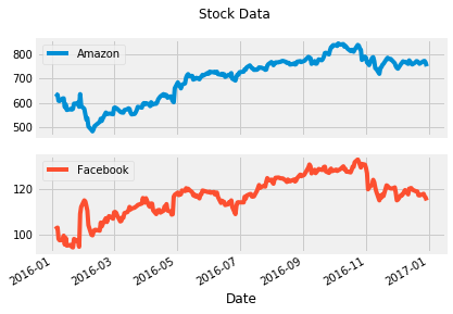
Plot & summarize daily prices for Amazon and Facebook
Before we compare an investment in either Facebook or Amazon with the index of the 500 largest companies in the US, let's visualize the data, so we better understand what we're dealing with.
# visualize the stock_data
stock_data.plot(subplots=True, title='Stock Data')

# summarize the stock_data
stock_data.describe()
| Amazon | ||
|---|---|---|
| count | 252.000000 | 252.000000 |
| mean | 699.523135 | 117.035873 |
| std | 92.362312 | 8.899858 |
| min | 482.070007 | 94.160004 |
| 25% | 606.929993 | 112.202499 |
| 50% | 727.875000 | 117.765000 |
| 75% | 767.882492 | 123.902503 |
| max | 844.359985 | 133.279999 |
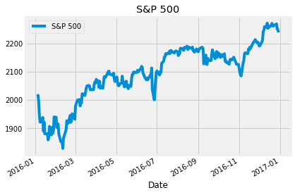
Visualize & summarize daily values for the S&P 500
Let's also take a closer look at the value of the S&P 500, our benchmark.
# plot the benchmark_data
benchmark_data.plot(title='S&P 500')

# summarize the benchmark_data
benchmark_data.describe()
| S&P 500 | |
|---|---|
| count | 252.000000 |
| mean | 2094.651310 |
| std | 101.427615 |
| min | 1829.080000 |
| 25% | 2047.060000 |
| 50% | 2104.105000 |
| 75% | 2169.075000 |
| max | 2271.720000 |
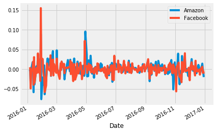
The inputs for the Sharpe Ratio: Starting with Daily Stock Returns
The Sharpe Ratio uses the difference in returns between the two investment opportunities under consideration.
However, our data show the historical value of each investment, not the return. To calculate the return, we need to calculate the percentage change in value from one day to the next. We'll also take a look at the summary statistics because these will become our inputs as we calculate the Sharpe Ratio. Can you already guess the result?
# calculate daily stock_data returns
stock_returns = stock_data.pct_change()

# plot the daily returns
stock_returns.plot()

# summarize the daily returns
stock_returns.describe()
| Amazon | ||
|---|---|---|
| count | 251.000000 | 251.000000 |
| mean | 0.000818 | 0.000626 |
| std | 0.018383 | 0.017840 |
| min | -0.076100 | -0.058105 |
| 25% | -0.007211 | -0.007220 |
| 50% | 0.000857 | 0.000879 |
| 75% | 0.009224 | 0.008108 |
| max | 0.095664 | 0.155214 |
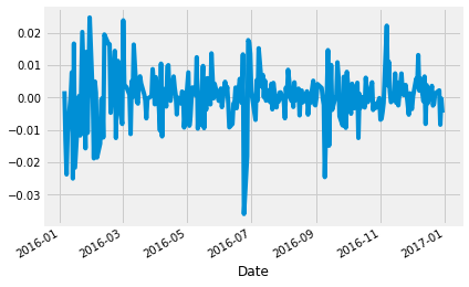
Daily S&P 500 returns
For the S&P 500, calculating daily returns works just the same way, we just need to make sure we select it as a Series using single brackets [] and not as a
DataFrame to facilitate the calculations in the next step.
# calculate daily benchmark_data returns
sp_returns = benchmark_data['S&P 500'].pct_change()

# plot the daily returns
sp_returns.plot()

# summarize the daily returns
sp_returns.describe()
Output
    count    251.000000
    mean       0.000458
    std        0.008205
    min       -0.035920
    25%       -0.002949
    50%        0.000205
    75%        0.004497
    max        0.024760
    Name: S&P 500, dtype: float64
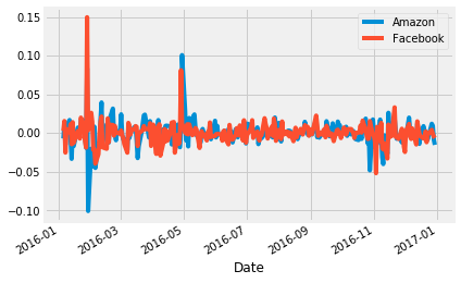
Calculating Excess Returns for Amazon and Facebook vs. S&P 500
Next, we need to calculate the relative performance of stocks vs. the S&P 500 benchmark. This is calculated as the difference in returns between stock_returns and
sp_returns for each day.
# calculate the difference in daily returns
excess_returns = stock_returns.sub(sp_returns, axis=0)

# plot the excess_returns
excess_returns.plot()

# summarize the excess_returns
excess_returns.describe()
| Amazon | ||
|---|---|---|
| count | 251.000000 | 251.000000 |
| mean | 0.000360 | 0.000168 |
| std | 0.016126 | 0.015439 |
| min | -0.100860 | -0.051958 |
| 25% | -0.006229 | -0.005663 |
| 50% | 0.000698 | -0.000454 |
| 75% | 0.007351 | 0.005814 |
| max | 0.100728 | 0.149686 |
The Sharpe Ratio
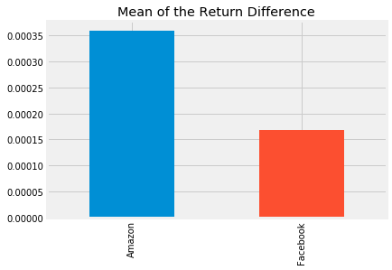
Step 1: The Average Difference in Daily Returns Stocks vs S&P 500
Now we can finally start computing the Sharpe Ratio. First we need to calculate the average of the
excess_returns. This tells us how much more or less the investment yields per day compared to the benchmark.
# calculate the mean of excess_returns
avg_excess_return = excess_returns.mean()

# plot avg_excess_returns
avg_excess_return.plot.bar(title='Mean of the Return Difference')
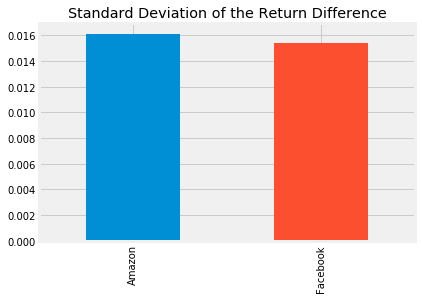
Step 2: Standard Deviation of the Return Difference
It looks like there was quite a bit of a difference between average daily returns for Amazon and Facebook.
Next, we calculate the standard deviation of the excess_returns. This shows us the amount of risk an investment in the stocks implies as compared to an investment in the S&P 500.
# calculate the standard deviations
sd_excess_return = excess_returns.std()

# plot the standard deviations
sd_excess_return.plot.bar(title='Standard Deviation of the Return Difference')
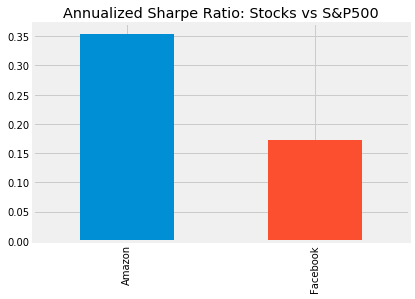
Putting it all together
Now we just need to compute the ratio of avg_excess_returns and
sd_excess_returns. The result is now finally the Sharpe ratio and indicates how much more (or less) return the investment opportunity under consideration yields per unit of risk.
The Sharpe Ratio is often annualized by multiplying it by the square root of the number of periods. We have used daily data as input, so we'll use the square root of the number of trading days (5 days, 52 weeks, minus a few holidays): √252
# calculate the daily sharpe ratio
daily_sharpe_ratio = avg_excess_return.div(sd_excess_return)

# annualize the sharpe ratio
annual_factor = np.sqrt(252)
annual_sharpe_ratio = daily_sharpe_ratio.mul(annual_factor)

# plot the annualized sharpe ratio
annual_sharpe_ratio.plot.bar(title='Annualized Sharpe Ratio: Stocks vs S&P500')
Conclusion
Given the two Sharpe ratios, which investment should we go for? In 2016, Amazon had a Sharpe ratio twice as high as Facebook. This means that an investment in Amazon returned twice as much compared to the S&P 500 for each unit of risk an investor would have assumed. In other words, in risk-adjusted terms, the investment in Amazon would have been more attractive.
This difference was mostly driven by differences in return rather than risk between Amazon and Facebook. The risk of choosing Amazon over FB (as measured by the standard deviation) was only slightly higher so that the higher Sharpe ratio for Amazon ends up higher mainly due to the higher average daily returns for Amazon.
When faced with investment alternatives that offer both different returns and risks, the Sharpe Ratio helps to make a decision by adjusting the returns by the differences in risk and allows an investor to compare investment opportunities on equal terms, that is, on an 'apples-to-apples' basis.
# Uncomment your choice.
buy_amazon = True
# buy_facebook = True